← worksCourse project · AI & Society202418/20
Exploring Data Complexity on the Wine Dataset
Analyzing the data complexity of the Wine dataset from scikit-learn and discussing its implications for Decision Trees, KNN, and SVM.
Adriano Machado · Faculty of Sciences, University of Porto
1. Introduction
To set appropriate expectations for classification performance, it is essential to understand the complexity of a specific dataset. This report aims to analyze the data complexity of the Wine dataset from SciKit-Learn and discuss its implications for classification algorithms such as Decision Trees, K-Nearest Neighbors (KNN), and Support Vector Machines (SVM).
2. Methodology
(1) Data Preprocessing: Certain complexity measures, such as F1 and F2, require normalized features. This was done by applying the StandardScaler from Scikit-Learn to standardize the feature set.
(2) Data Complexity Analysis: The Problexity library was used to compute several data complexity measures based on the work of Garcia et al. (2018). These measures were categorized into:
- Feature Overlapping Measures
- Linearity Measures
- Neighborhood Measures
- Dimensionality Measures
- Class Balance Measures
(3) Principal Component Analysis: to assess instance hardness and the distribution of instances in the feature space, we used the Pyhard library to plot the Principal Component Analysis (PCA) graph.
(4) Classifier Evaluation: Following the complexity analysis, we split the dataset into training and test sets. GridSearchCV was used for hyperparameter tuning of the three chosen classifiers (Decision Trees, KNN, and SVM), optimizing their parameters for each model to ensure fair performance comparison. The classifiers were evaluated based on metrics such as accuracy, precision, recall, and F1-score, allowing us to analyze how well each classifier performed in light of the dataset’s complexity.
3. Results and Discussion
3.1 Data Complexity Analysis
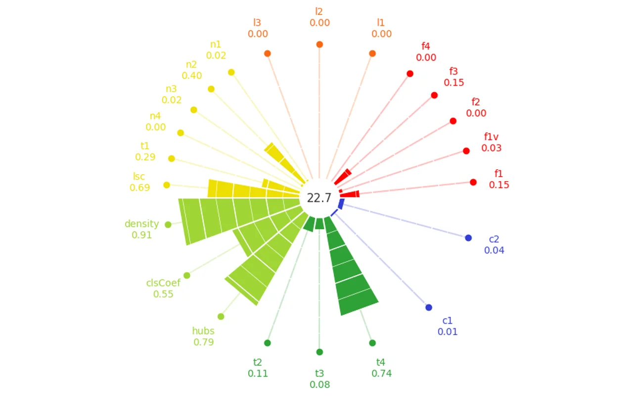
The complexity measures, as visualized in Figure 1, revealed several characteristics.
Low Feature Overlap: The very low values for F1, F1v, F2, F3, and F4 (red) suggest that there is little to no overlap between classes in the feature space. This implies that the features are highly discriminative and can effectively separate the classes.
Linear Separability: The near-zero values for L1, L2, and L3 suggest that the classes are linearly separable, making linear classifiers a suitable choice.
Neighborhood Structure: The neighborhood measures suggest clear class separation with minimal boundary regions (N1 = 0.02) and perfect local linearity (N4 = 0.00). While there is some spread in the feature space (T1 = 0.29), the high local set cardinality (LSC = 0.69) indicates dense class neighborhoods. These characteristics suggest both distance-based and linear classifiers should perform well on this dataset.
Network Structure: The high density (0.91) suggests sparse connectivity between instances, although a moderate clustering coefficient (0.55) indicates some local grouping. The hub score (0.79) suggests the presence of well-connected nodes within the class structures.
Dimensionality: Low T2 (0.11) and T3 (0.08) values indicate a non-sparse dataset with manageable complexity. The high T4 value (0.74) suggests most original features are important for maintaining data variability.
Class Balance: The extremely low values of C1 (0.01) and C2 (0.04) indicate well-balanced classes, suggesting that class imbalance will not be a significant challenge for classification algorithms.
3.2 Principal Component Analysis
The PCA plot shows three partially overlapping clusters representing the three classes of the target variable distributed across the feature space. While most instances appear in blue indicating they are easier to classify, the red-colored points tend to occur at cluster boundaries and overlap regions. This suggests that the dataset has some instances that are harder to classify due to their proximity to other classes.
3.3 Implications for Classification Algorithms
The complexity measures show good conditions for all three classifiers, though each has its own advantages. Support Vector Machines (SVM) are likely to perform great due to the high linear separability and low feature overlap, allowing for optimal hyperplane placement with clear margins between classes. The K-Nearest Neighbors benefits from the clear neighborhood structure and minimal boundary regions although the sparcity of the network may affect its performance. For Decision Trees, the low feature overlap measures (F1-F4) indicate that effective splitting criteria can be identified, but the high T4 value (0.74) suggests that multiple features may be needed for optimal splits, potentially leading to deeper trees.
3.4 Classification Algorithms Comparison
The previous conclusions about the complexity metrics are corroborated by the performance of the three classifiers.
- SVM (Support Vector Machine) achieved the highest accuracy (0.98), which matches the dataset’s linear separability and low complexity.
- KNN (K-Nearest Neighbors) came in second with an accuracy of 0.96, benefiting from the clear class neighborhoods. However, network sparsity may have slightly impacted its performance compared to SVM.
- Decision Trees were third with an accuracy of 0.94. Despite the dataset’s linear separability, potential overfitting may have limited its performance.
| Classifier | accuracy | precision |
|---|---|---|
| Decision Tree | 0.944444 | 0.951389 |
| K-Nearest Neighbors | 0.962963 | 0.965123 |
| Support Vector Machine | 0.981481 | 0.982716 |
Table 1: Performance metrics of classification algorithms
4. Conclusions
The complexity measures employed in this study provided valuable informations about the characteristics of our dataset. These metrics allowed us to identify key properties that informed our understanding of which classification algorithms were likely to perform well and why some algorithms might underperform. The conclusions drawn from these metrics were validated when we tested the performance of our models.
References
[1] Luís P. F. Garcia, Ana C. Lorena, Marcilio C. P. de Souto, and Tin Kam Ho. 2018. Classifier Recommendation Using Data Complexity Measures. In 2018 24th International Conference on Pattern Recognition (ICPR). IEEE, 591–597. https://doi.org/10.1109/ICPR.2018.8545249
[2] Joanna Komorniczak and Paweł Ksieniewicz. 2023. problexity—An open-source Python library for supervised learning problem complexity assessment. Neurocomputing 521 (2023), 126–136.
[3] A. C. Lorena, L. P. Garcia, J. Lehmann, M. C. Souto, and T. K. Ho. 2019. How complex is your classification problem? A survey on measuring classification complexity. ACM Computing Surveys (CSUR) 52, 5 (2019), 1–34. https://doi.org/10.1145/3347711
[4] P. Y. A. Paiva, K. Smith-Miles, M. G. Valeriano, and A. C. Lorena. 2021. PyHard: A novel tool for generating hardness embeddings to support data-centric analysis. arXiv preprint arXiv:2109.14430 (2021). https://arxiv.org/pdf/2109.14430
